
This note primarily delves into the dispersion relation and solutions of the water wave equation incorporating surface tension.
One Dimensional Waves with Surface Tension
surface tension is included \[ \frac{2 \pi \eta}{P}=\lim _{\epsilon \rightarrow 0}\left\{\int_0^{\infty} \frac{e^{i \kappa x_1} d \kappa}{\kappa U^2-2 i \epsilon U-g-(T / \rho) \kappa^2}+\int_0^{\infty} \frac{e^{-i \kappa x_1} d \kappa}{\kappa U^2+2 i \epsilon U-g-(T / \rho) \kappa^2}\right\} \] The poles are \[ k U^2=g+\frac{T}{\rho} k^2 \] phase velocity \[ U=c(k) \] When \(U<c_m\), where \(c_m\) is the minimum wave speed, the zeros are not real. When \(U>c_m\), there are two real roots \(k_{\mathrm{g}}\) and \(k_T\), with \(k_T>k_{\mathrm{g}}\). In this case, \[ \kappa=k_g+\frac{2 \rho U}{\left(k_T-k_g\right) T} i \epsilon, \quad \kappa=k_T-\frac{2 \rho U}{\left(k_T-k_g\right) T} i \epsilon \] The asymptotic wavetrains are \[ \eta \sim \begin{cases}\frac{-2 P \rho}{\left(k_T-k_g\right) T} \sin k_g x_1, & x_1>0, \\ \frac{-2 P \rho}{\left(k_T-k_g\right) T} \sin k_T x_1, & x_1<0 .\end{cases} \] this indicate that gravity waves downstream and capillary waves upstream.
ship waves
for 2-d gravity waves, and pressure source \(f\left(x_1, x_2\right)=P \delta\left(x_1, x_2\right)\), the fourier transform is \(F(\kappa)=P / 4 \pi^2\) \[ \frac{4 \pi^2 U^2 \eta}{P}=e^{\epsilon t}\int_{-\infty}^{\infty} \int_{-\infty}^{\infty} \frac{\kappa \exp \left\{i\left(\kappa_1 x_1+\kappa_2 x_2\right)\right\} d \kappa_1 d \kappa_2}{\left(\kappa_1-i \epsilon / U\right)^2-g \kappa / U^2} \]
Unsolved
\[\begin{aligned}\int_{-\infty}^{\infty} \int_{-\infty}^{\infty} &\frac{\kappa \exp \left\{i\left(\kappa_1 x_1+\kappa_2 x_2\right)\right\} d \kappa_1 d \kappa_2}{\left(\kappa_1 U-i \epsilon\right)^2-\omega_0^2(\kappa)}\\&=\int_{-\infty}^{\infty} \frac{\kappa F(\boldsymbol\kappa) e^{i \boldsymbol\kappa \cdot \boldsymbol x} d \boldsymbol\kappa}{\left(\kappa_1 U-i \epsilon\right)^2-\omega_0^2(\kappa)}\end{aligned}\] why does \(d \boldsymbol\kappa=d \kappa_1 d \kappa_2\)?
where \(\kappa=\left(\kappa_1^2+\kappa_2^2\right)^{1 / 2}\), we introduce a polar coordinates \[
\begin{array}{ll}
x_1=r \cos \xi, & x_2=r \sin \xi \\
\kappa_1=-\kappa \cos \chi, & \kappa_2=\kappa \sin \chi
\end{array}
\] The contribution from the range \(\pi / 2<\chi<3 \pi / 2\) is the conjugate of the range \(-\pi / 2<\chi<\pi / 2\), and in the limit \(\epsilon \rightarrow 0\), then we have \[
\frac{2 \pi^2 U^2 \eta}{P}=\Re\left(\lim _{\epsilon \rightarrow 0} \int_{-\pi / 2}^{\pi / 2} \frac{d \chi}{\cos ^2 \chi} \int_0^{\infty} \frac{\kappa \exp \{-i \kappa r \cos (\xi+\chi)\}}{\kappa-\kappa_0} d \kappa\right)
\] where \[
\kappa_0=\frac{g}{U^2 \cos ^2 \chi}-\frac{2 i \epsilon}{U \cos \chi}
\] for arbitrary \(\chi_1 \in\left(\frac{\pi}{2}, \frac{3 \pi}{2}\right)\quad \exists \chi_2 \in\left(-\frac{\pi}{2}, \frac{\pi}{2}\right)\), and thus \(e^{i k \chi_1}=e^{-i k \chi_2} \rightarrow\) conjugate \[\int_0^{\infty} \frac{k e^{-i k r \cos (\xi+x)}}{k-k_0} d k\] simply it \[\int_0^{\infty} \frac{k e^{-i m k}}{k-k_0} d k\] where \(m=r \cos \left(\xi+x\right), k_0\) is the poles, and only focus on the contribution of poles \[\begin{aligned}& \int_c \frac{k e^{-i m k}}{k-k_0} d k=2 \pi i \operatorname{Res}\left[f(z), z_0\right] \\\\& \operatorname{Res}\left[f(z), z_0\right]=\lim _{z \rightarrow z_0}\left(z-z_0\right) f\left(z_0\right) \text { ( for 1st pole) }\end{aligned}\] \(k_0\) is the first-order pole, then \[\underset{k=k_0}{\operatorname{Res}} \left[f(k)\right]=k_0 e^{-i m t_0}\]notes
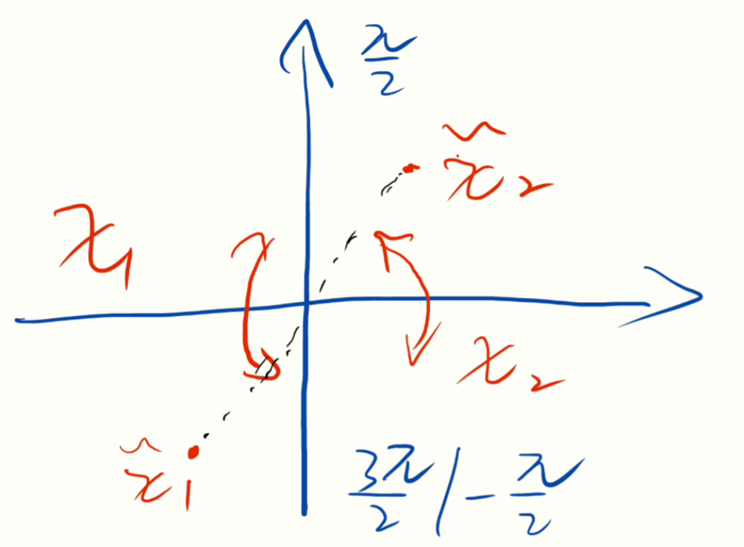
\(\left\{\begin{array}{l}\cos \chi_1=-\cos \chi_2 \\ \sin \chi_1=-\sin \chi_2\end{array}\right.\) notes